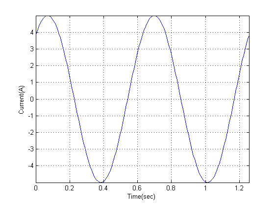
How do I plot a sinusoidal equation with MATLAB?

You've seen pretty graphs everywhere. Maybe you wonder how to make them. Maybe you're just stuck on a problem you must solve with MATLAB. Regardless, you've come here for answers. This article plots a sine wave in MATLAB that displays two cycles that automatically scale according to your equation. If you've never used MATLAB before, I recommend reading a primer article first.

In case you didn't know, MATLAB is a great tool for graphing equations.

Let's look at what I entered to get the above graph and break it down step by step. First, open MATLAB and get to the command prompt. If you were already doing something, type "clear" to clear your variables. Type "clc" to clear your command line. It's therapeutic. Kind of. Now we type:

>> v=34exp(j125pi/180);

This code is the same as saying that v is the same as the phasor notation 34 phase 125. If you're not an electrical engineer, don't worry about that too much. Phasors are discussed in a separate article. They're a convenient way of giving a frequency-independent description of a sine wave's amplitude and phase angle displacement. In this case, we're saying that the amplitude is 34 and the phase displacement is 125 degrees.

>> omega = 10;

Ok, we're setting our frequency variable to 10 radians per second

>> T = 2pi/omega;

This defines T as your period for your wave.

>> delta_t=T/100;

By using variables in our scaling, we can easily reuse this code. delta_t will be our steps from each dot on the graph to the next. Think of it as your sample size. Note that we're going to take 100 samples per period.

>> t=0:delta_t:2T;

The variable "t" will be used for our values to plot from. This code generates a matrix from 0 up to 2T in steps of T/100. If you want more points plotted for a smoother graph, make your delta_t value smaller. This will cause your code to take longer to execute, however. If you wanted to have more spacing along the top and bottom of the graph, set this without using any variables. However, you lose your automatic scaling by doing that.

>>v_t=abs(v)cos(omegat+angle(v));

Here's the equation we entered earlier coming back into play. Translating this code into English, we're taking the phasor "v" and calculating the magnitude of the phasor. This is equal to the square root of the summation of the phasor's rectangular form. It's just sqrt(a^2+b2), so don't panic. After that, we're multiplying our frequency by our calculated values in matrix "t" over the two cycles, then shifting that by our phase angle. It's a standard sinusoid, so we're using cosine. If we decided to use sine instead of cosine, you'd have to enter a "v" value at an angle 90 degrees less than what we did above. That means instead of 34 phase 125, it would be 34 phase 35.

>> plot(t,v_t)

This command finally plots our equation using those two variables as our independent and dependent variables.

>> grid

Everyone likes a nice grid, right?

>> axis([0 2*T -Inf Inf])

This sets the axis spacing according to this format: [xmin xmax ymin ymax]
What this does is set up the last thing we need for our scaling only to have two cycles of our sine wave. The -Inf and Inf let the y axis be as high as it needs to be to contain all points.

>> ylabel('Voltage(V)')
>> xlabel('Time(sec)')

These two lines of code label the y and x axes, respectfully. Note that what you want the label to be must be enclosed in single quotes.

Now, believe it or not, you're done and have a nicely formatted sinusoidal wave.

Matlab is a copyrighted of The MathWorks, Inc. Purchase MATLABÂ here.
Wirebiters.com and The Math Works, Inc are not affiliated in any way.